
The Large Hadron Collider (LHC) is one of the most sophisticated experiments ever designed. Its primary purpose is to probe the internal structures of matter and study the underlying physics and interactions of the particles that make up our universe. Particles collide at LHC at a rate of 40 MHz, generating vast amounts of data every second. The collisions are recorded at 4 four interaction points where a sophisticated detector is located. The Compact Muon Solenoid (CMS) Experiment is one such detector.CMS generates data at a theoretical throughput of
Level-1 Trigger The first triggering stage reduced the event rate from 40 MHz to a maximum of 110 kHz, considering the data rate and timing constraints, as well as the hardware constraints of FPGAs. The L1 Trigger can only run a course reconstruction of the incoming physics events, given that it receives only a fraction of the total event-level information from the detector and heavily depends on cut-based algorithms that can introduce significant physics biases within the trigger system.
High-Level-Trigger The second stage of the triggering system (HLT) further reduces the event rate from 100 kHz to around 1 kHz, at which point the data can be permanently stored. The HLT receives complete information from the entire detector, enabling a comprehensive physics reconstruction.
Traditionally, physics-based algorithms were used in the triggering system. However, given the massive success of machine learning (ML) and deep learning, it is essential to investigate whether an ML-based algorithm can enhance the triggering system. Since most of the triggering system is based on FPGA-based computational hardware, computational footprint and timing constraints should also be taken into account. This work demonstrates how ML-based triggering algorithms can be designed that are both computationally lighter and have superior performance compared to traditional physics-based algorithms on tasks such as online recalibration of physics objects and classification of dimuon pairs.
Various metrics are used to compare the performance (in terms of computational cost) and resolution (in terms of prediction accuracy) of different models. The following metrics are defined that will be used extensively later on.
Hardware Values: Hardware values are the data received from the detector and used by the L1-Trigger to make decisions. Reconstructed Values: Reconstructed values are the corrected values that are calculated after a full physics reconstruction. Reconstructed values are not available on the L1-Trigger.
Regression
For regression tasks, the metric employed is the Full-Width-Half-Maximum (FWHM), which reads:
Classification For classification tasks, the Area Under the Receiver Operating Characteristic curve (AUC-ROC) score is chosen as a metric.
Where:
-
$\mathrm{TPR} = \frac{\mathrm{TP}}{\mathrm{TP} + \mathrm{FN}}$ is the True Positive Rate -
$\mathrm{FPR} = \frac{\mathrm{FP}}{\mathrm{FP} + \mathrm{TN}}$ is the False Positive Rate
Computational and Hardware Cost
To measure the computational cost of our model on the FPGAs, we will use the following metrics:
Digital Signal Processors (DSP): DSP chips are used for processing the relevant signals coming to the FPGA board, particularly additions and multiplications. Flip-Flops (FF): These units help synchronize logic and save logical states between clock cycles within an FPGA circuit. Look-up-Tables (LUT): These units help in implementing arbitrary Boolean logics inside the FPGA. textbf{Block RAM (BRAM): a type of random access memory implemented inside the FPGA for data storage.
The number of these resources available is minimal. Hence, models with the least amount of resource consumption are given a higher priority.
Recalibrating of
A four-layer neural network with 256 neurons in each layer is chosen as the teacher model. ReLU non-linearity is used in conjunction with batch normalization after every subsequent layer. The output layer consists of three parameters that predict the recalibrated
A four-layer neural network with eight neurons in each layer is chosen as the student model. ReLU non-linearity is used in conjunction with batch normalization after every subsequent layer. The output layer consists of three parameters that predict the recalibrated
To compare the effectiveness of the proposed method, the above models are evaluated against existing baselines in terms of both reconstruction resolution and computational requirements. The reported model from 1 is used as the baseline for this study. The model is a four-hidden-layer neural network with 16 neurons in each layer trained with a similar loss and schedule as the teacher model.
| FWHM | Teacher | Student | Baseline |
|---|---|---|---|
| 0.120 | 0.1240 | 0.140 | |
| 0.061 | 0.063 | 0.0662 | |
| 0.413 | 0.417 | 0.433 |
The table above shows the performance of the three models across the three parameters
Although the student model is approximately 1024 times smaller than the teacher, it performs almost as well, outperforming the baseline by a large margin despite being four times lighter.
| VU9P FPGA | DSP | Flip Flops | Look Up Table | BRAMs |
|---|---|---|---|---|
| Available | 9024 | 2.6 M | 1.3 M | 2160 |
| Student | 72 (0.79%) | 5677 (0.21%) | 11.3 K (0.87%) | 0 |
| Baseline | 238 (2.61%) | 11.6 K (0.43%) | 33.2 K (3.38%) | 0 |
The table above shows the usage of various units of a VU9P FPGA when each model is run on it. The DSP reuse factor is set to 4 for all the experiments. Clearly, the student is much lighter compared to the pre-existing baseline.
Although the student model outperforms the baseline across all metrics, a deeper understanding of its performance is still required before moving forward. This section examines the recalibration model (student) in detail. The resolution peaks for each kinematic quantity are plotted in the figure below. From the plot, it can be inferred that the model performs well against
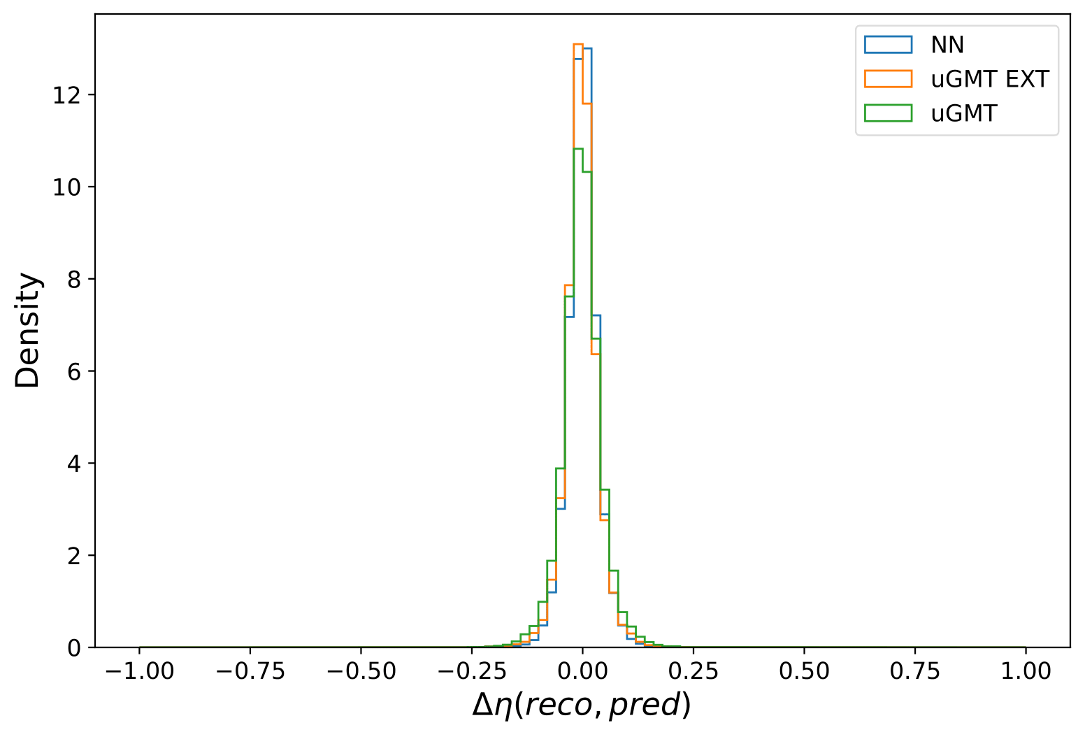
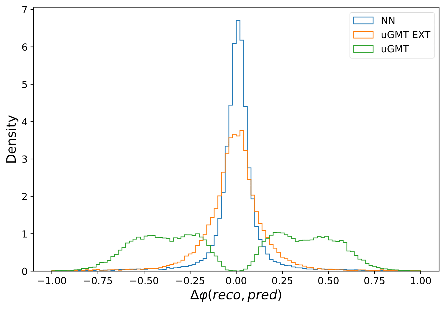
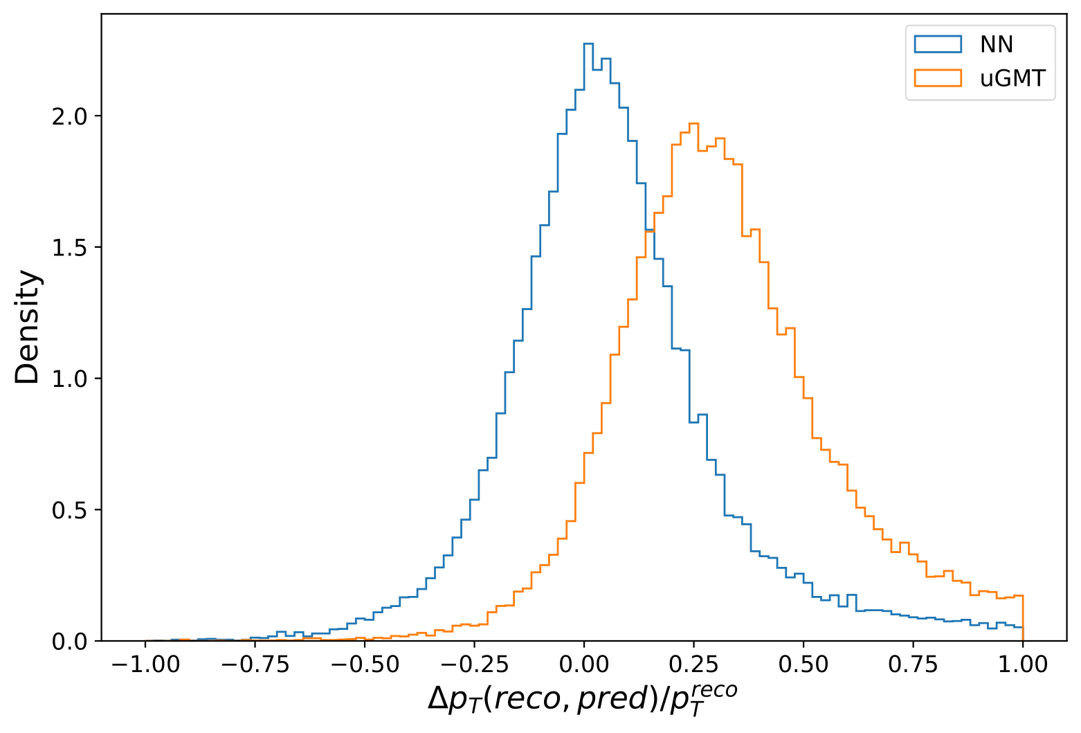
In the above plot,
Next, the resolution of recalibrated
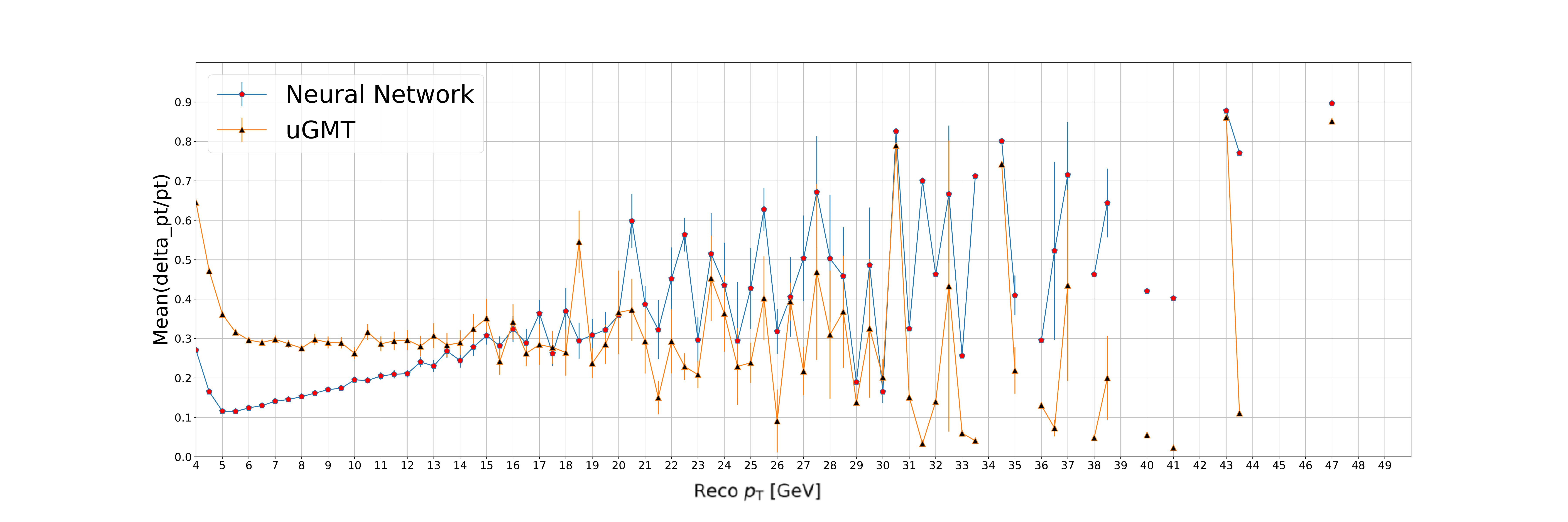
Plotting the resolution of recalibrated
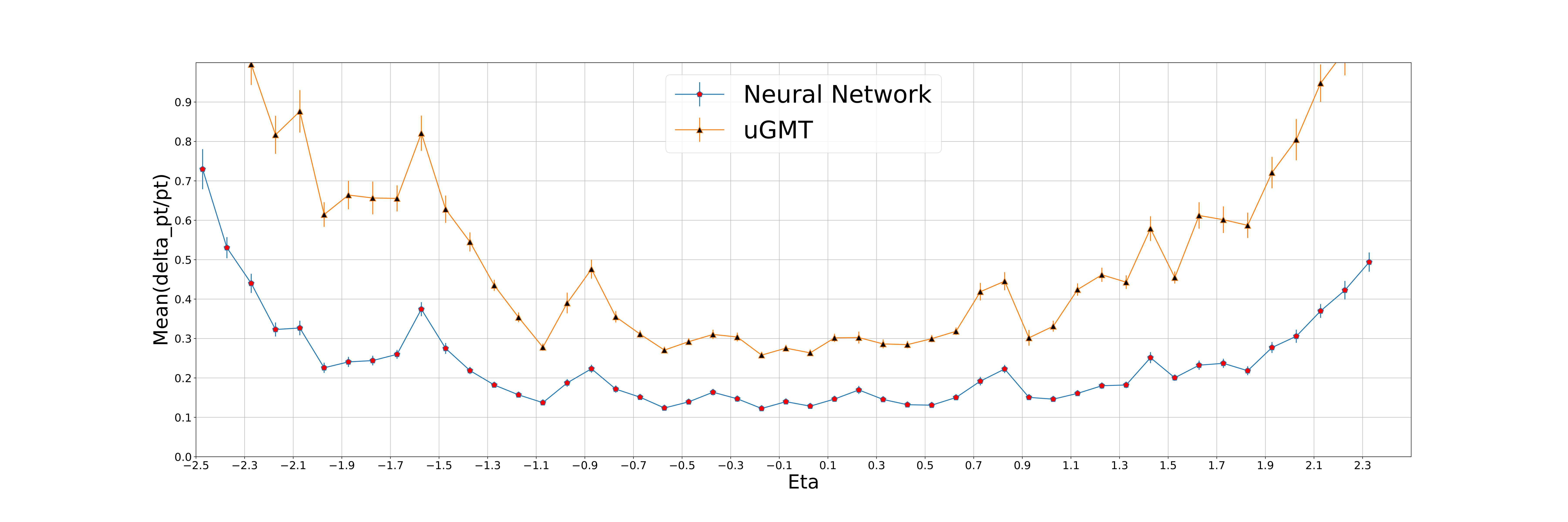
The reason behind the poor recalibration performance of the ML model at the high
- Presence of exponentially fewer samples in the high
$p_T$ region, given that it corresponds to high-energy collisions that occur less frequently. - High
$p_T$ samples bend significantly less in the magnetic field present within the CMS detector, making their momentum harder to estimate within the muon chamber, making them more error-prone.
Although the model performs very well for low to moderate
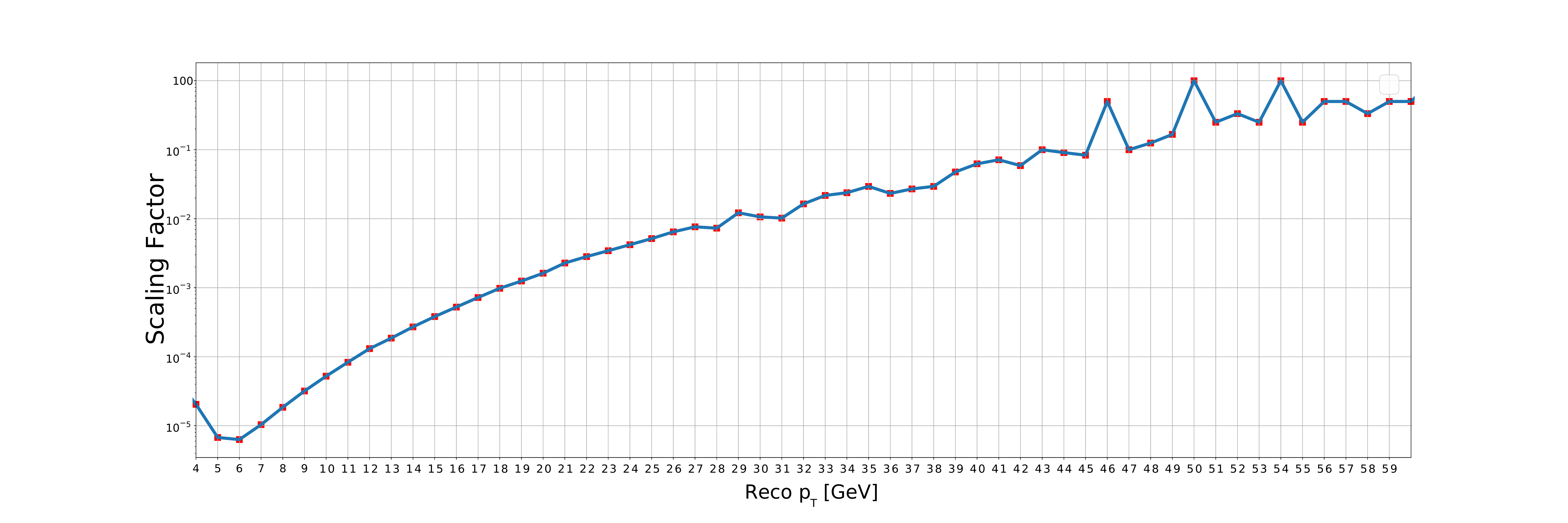
- Loss Scaling: The loss is scaled to incentivise the model to work better for the high
$p_\mathrm{T}$ region. The loss is scaled to the inverse of the number of samples in the dataset, in bins of size 1, with similar$p_\mathrm{T}$ values during the distillation step. - Two Models: Since the model starts to perform worse for high reco
$p_\mathrm{T}$ , intuitively, one might think that using two models, one for the low reconstructed$p_\mathrm{T}$ region and the other for the reconstructed high$p_\mathrm{T}$ region, should be sufficient to solve the problem. Hence, a two-model approach is also chosen and experimented with.
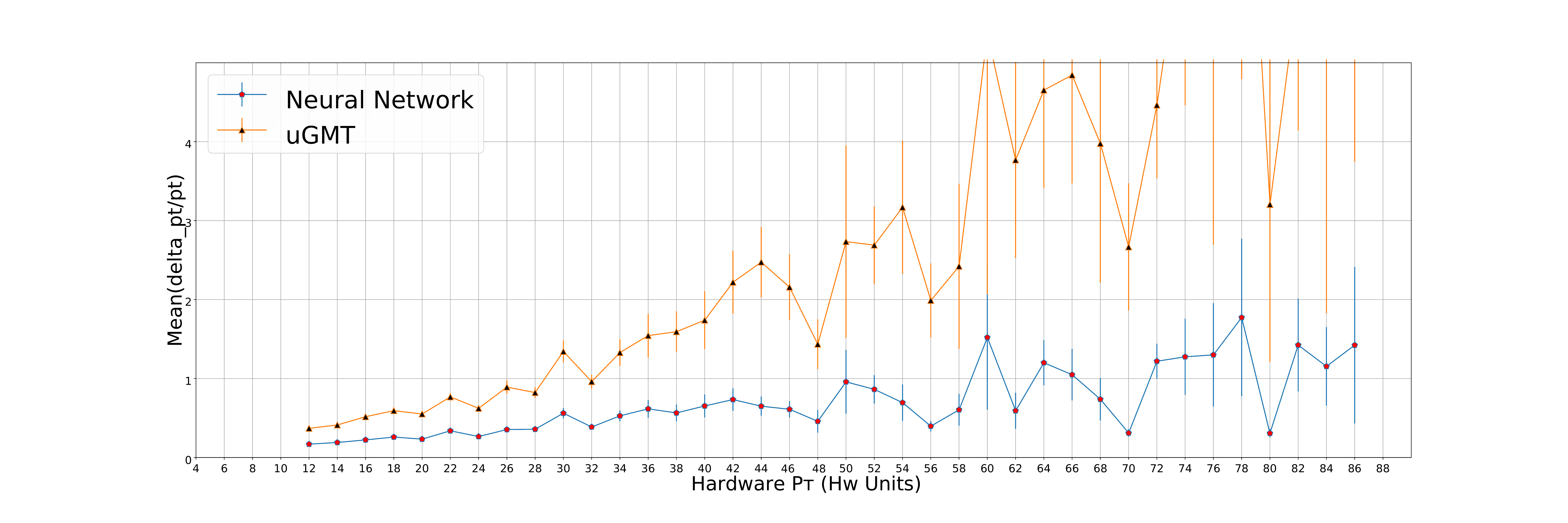
Plotting the resolution vs. the reco 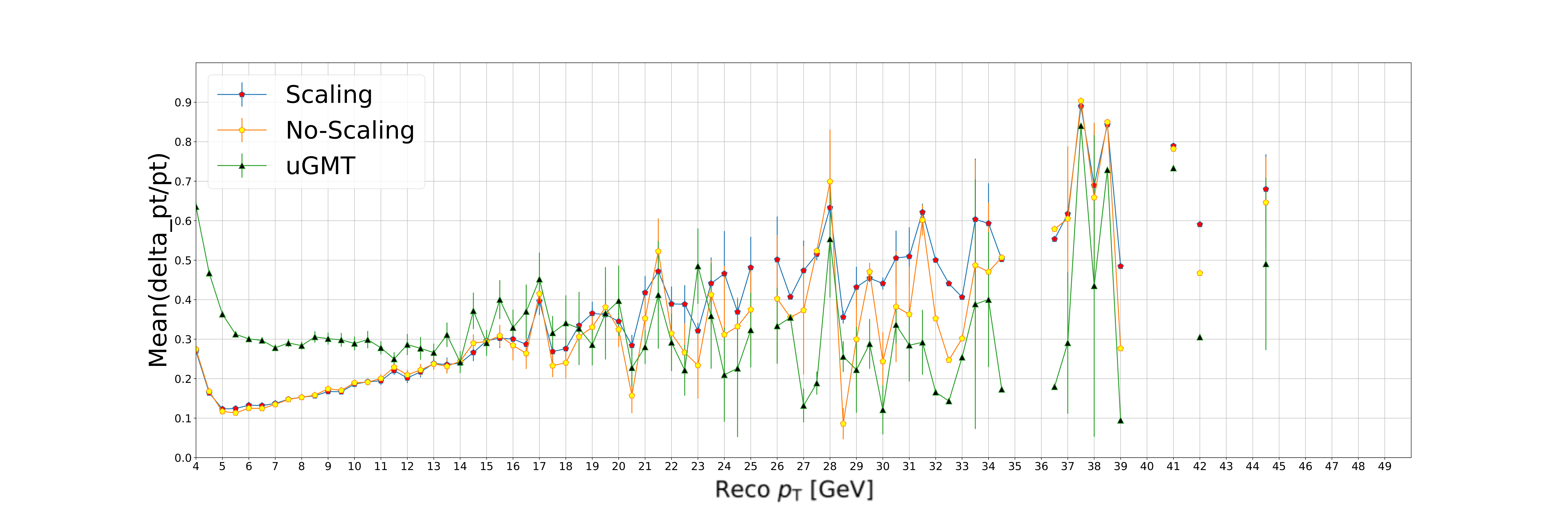
Next, the two models approach is explored. The figure below shows the resolution vs reco
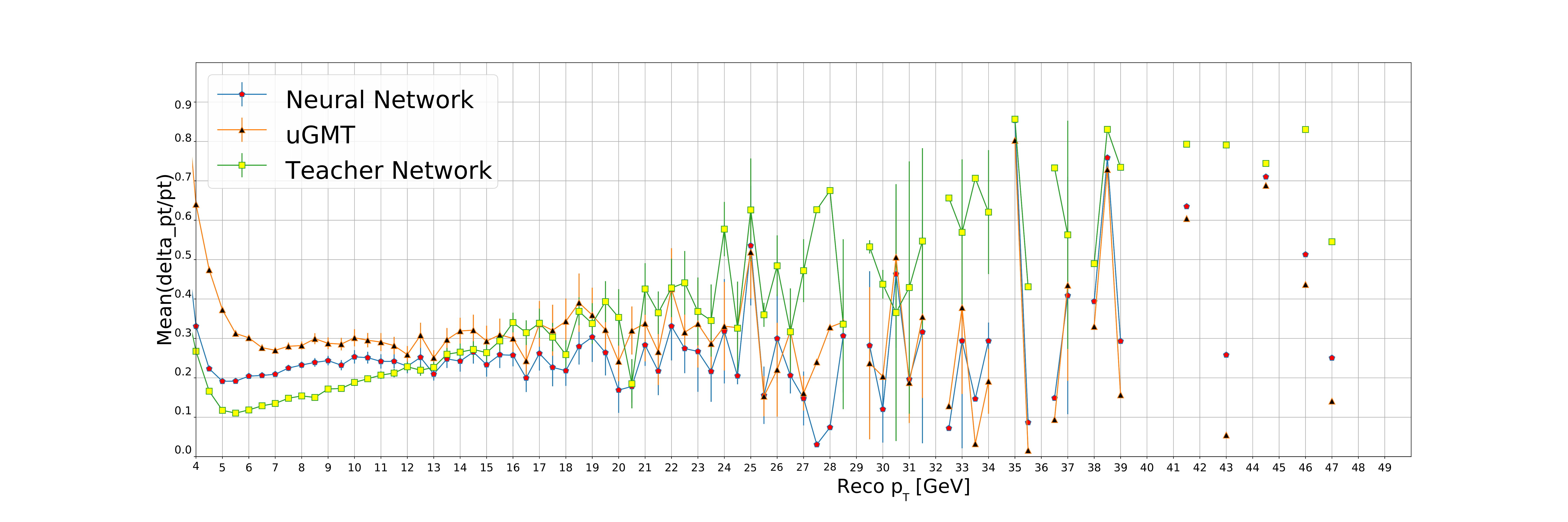
This is not because the model lacks learning capabilities. The low resolution in the high
Next, the interest lies in predicting whether a di-muon pair can be identified from a chosen pair of muons using the L1 parameters
A four-layer neural network with 256 neurons in each layer is chosen as the teacher model. ReLU non-linearity is used in conjunction with batch normalization after every subsequent layer. The output layer consists of a single neuron with linear/no activation. QKeras is used to train the model with QAT precision fixed at [18,6]. The model is trained for 100 epochs using BinaryCrossEntropy (with logits) loss, and the learning rate is reduced after the model performance plateaus. Adam optimiser is used with an initial learning rate of
A four-layer neural network with eight neurons in each layer is used as a student model. ReLU non-linearity is used in conjunction with batch normalization after every subsequent layer. The output layer consists of a single neuron with linear/no activation. QKeras is used to train our model with QAT precision fixed at [18,6]. The model is trained for 500 epochs using BinaryCrossEntropy (with logits) as the task-agnostic loss and KLDivergence as the distillation loss. The distillation parameter
A model identical to the student model is trained just using BCE Loss (without distillation) as a control. All other parameters are kept identical to those of the student model trained in the previous step.
| Metric | Teacher | Student | Student (Non‑Distilled) |
|---|---|---|---|
| AUC‑ROC | 0.970 | 0.964 | 0.946 |
| AUC‑PR | 0.887 | 0.868 | 0.850 |
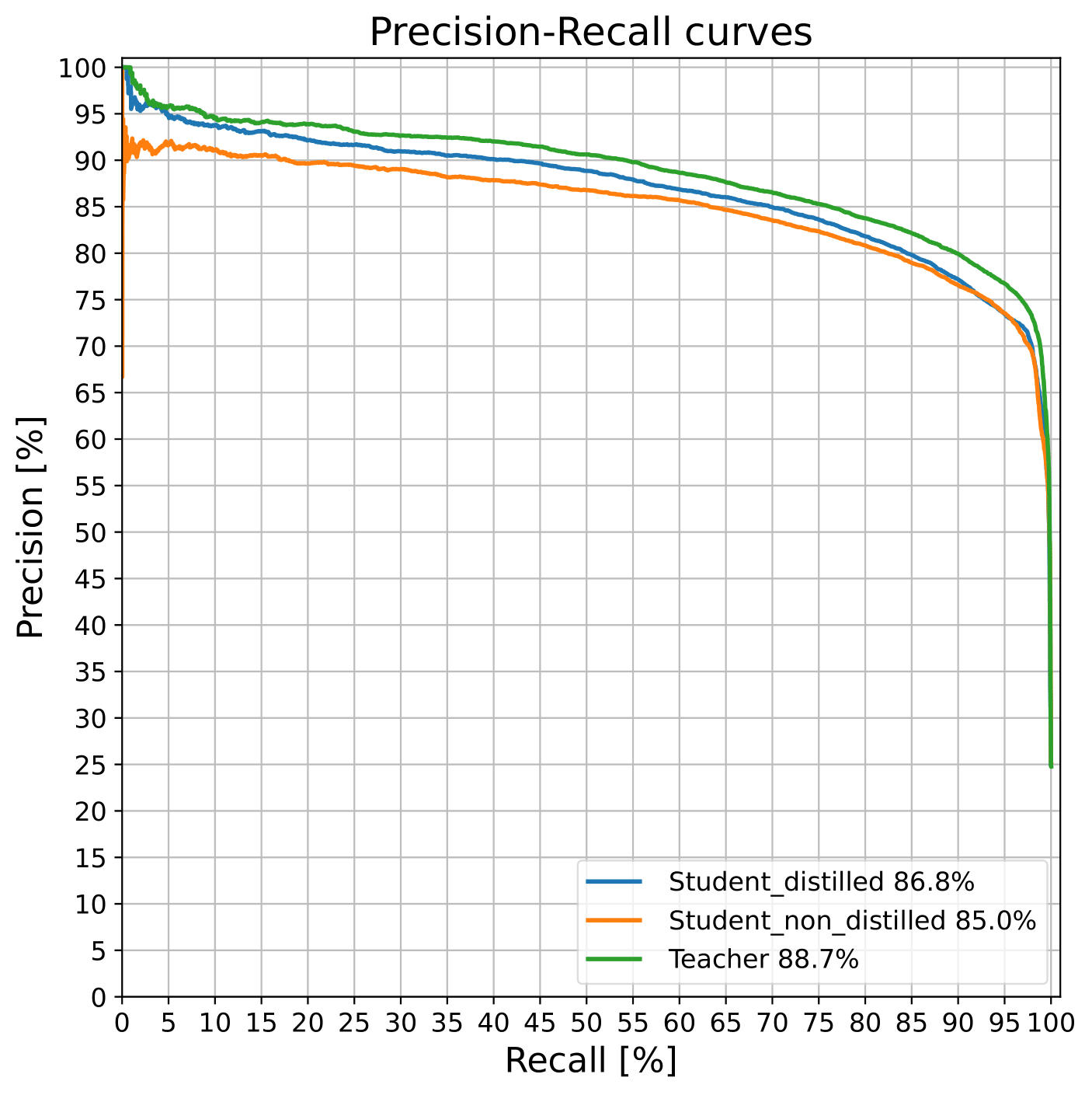
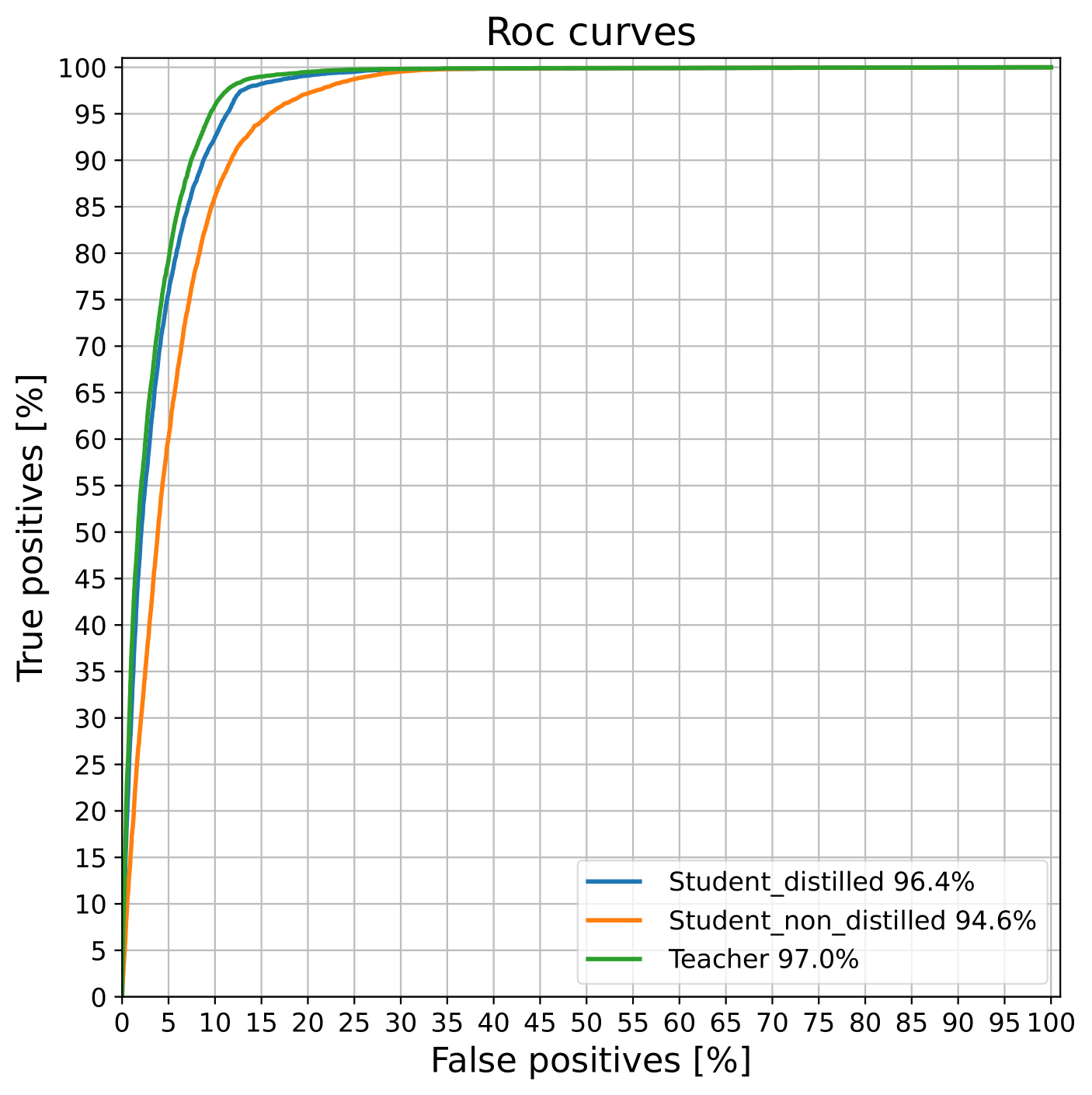
The table above shows the performance of the three models. Although the student model is much smaller than the teacher, it performs almost as well while being 1024 times lighter. It also outperforms the non‑distilled version, demonstrating the advantage of knowledge distillation.
| VU9P FPGA | DSP | Flip Flops | Look Up Tables | BRAMs |
|---|---|---|---|---|
| Available | 9024 | 2.6 M | 1.3 M | 2160 |
| Student | 78 (0.86 %) | 6110 (0.23 %) | 12.2 K (0.94 %) | 0 |
The table above shows the usage of various units of a VU9P FPGA when each model is deployed.
The DSP reuse factor is set to 4 for all experiments. The student model is clearly far lighter while maintaining competitive performance.
The PR and ROC curves are plotted in the figure below, where it can be seen that, for both metrics, the distilled model outperforms the non-distilled one by a considerable margin. Moreover, the information loss during the transfer of knowledge from the teacher to the student appears minimal, as the performance difference between the teacher and the distilled student is small.
In this work, various compression strategies have been explored to implement a lightweight neural network capable of delivering state-of-the-art performance, deployable on FPGA hardware systems in the CMS Level-1 trigger. A technique has been developed employing strategic combinations of quantization-aware training, knowledge distillation, and transfer learning to create a computationally efficient model with negligible loss in performance. The technique is tested on both classification and regression tasks, including $\mu$GMT muon recalibration and $\mu$GMT di-muon classification. The model outperformed the baseline significantly in the muon recalibration task, even after reducing the computational footprint fourfold. However, the model encountered challenges in the high reconstructed